For each scene and view, we provide a pair of undistorted stereo images, a depth map corresponding to the left image of the stereo pair, and where applicable a motion artefact mask. The mask identifies regions where scene motion occurred between capture of the LiDAR data, and capture of the stereo pairs (see Figure 1).

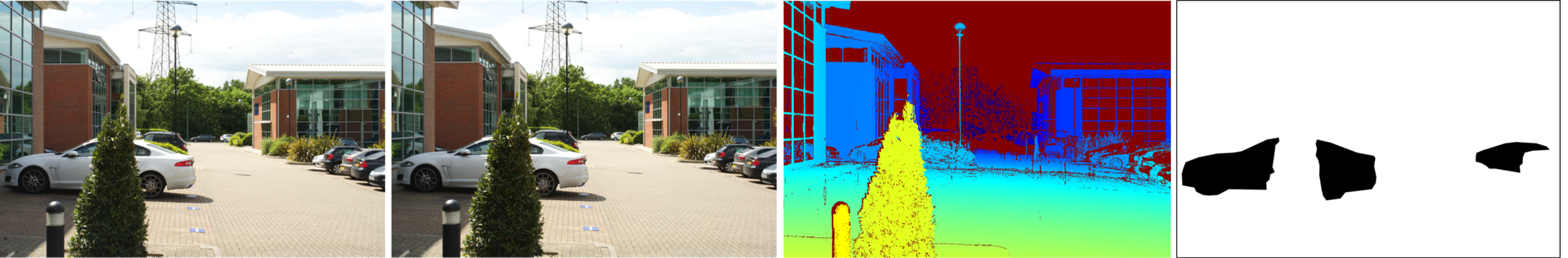
Figure 1. Example from Scene 18, View 6. Right and left stereo images, for cross-fusing, the depth map from LiDAR (colour gives range), and a motion mask. In this scene, one car appeared and another disappeared between the LiDAR and stereo image capture. Many scenes do not contain significant scene motion, and therefore no mask is supplied.  Scenes were captured on calm days, to minimise motion of vegetation in a breeze.

Some scenes / views are excluded from the stereo-LiDAR co-registered dataset because there were insufficient visual image features to provide good co-registration (see below). The range map and motion mask correspond to the left eye’s image in each pair. Stereo images have been undistorted using the estimated camera model from calibration images. The files containing the cameras’ models are left_cameraParams.mat and right_cameraParams.mat

The data are available at two scales. (i) Lower resolution, 600 x 900. All pixels have assigned depth except for those corresponding to LiDAR non-returns (e.g. sky, sea). (ii) Higher resolution, 688 x 1032. These include more LiDAR points, but a small number of pixels in the periphery have undefined depth due to differences between the spatial resolution and projection geometry of stereo images and the LiDAR data.  Where depth is undefined (for any reason) the depth map value is NaN.

Note: For scene 1, synchronisation between stereo cameras was poorer (up to 65msec) than for later scenes (max. 6msec). This can be seen in the stereo images of Scene 1, view 11 where the woman near the bus-stop has moved slightly between the left and right stereo image capture, and in view 12, the tops of the (mostly occluded) oncoming cars are mis-matched.

Details of co-registration

For each scene in the SYNS database, three types of data were recorded: an HDR image panorama, a LiDAR depth panorama, and 18 pairs of stereo images.  Here we describe the process of co-registration of the stereo pairs with the LiDAR depth information, all named functions are from Matlab (Mathworks).  As described elsewhere (Adams et al., 2016), the HDR and LiDAR data were obtained from a nominally common vantage point and were co-registered with the aid of 3 high-contrast co-registration targets placed in each scene.  The nodal points of the stereo cameras were positioned either side (±3.15cm horizontal offset) of the other two devices.  In order to co-register the stereo images with the LiDAR, the stereo images (the left eye’s view for each stereo pair) were first co-registered with the HDR panorama, via the steps described below.

Step 1

Panorama-Stereo alignment: The approximate correspondence between the 18 left eye images of the stereo pairs and the central strip of the HDR panorama was found. First, the (highly skewed) intensity distribution of the panorama was clipped to its 80^th centile, and the stereo images were resized (down-sampled) such that the two images shared the same average scale. For this stage it was unnecessary to remove/equate the distortions due to the different lenses of the two camera systems. The best azimuth alignment was found that maximised the correlation between the RGB values of the panorama and the 18 left eye stereo images. Because the angular separation between each of the 18 stereo views was known (20˚) this co-registration was a 1D search for a single rotation value.

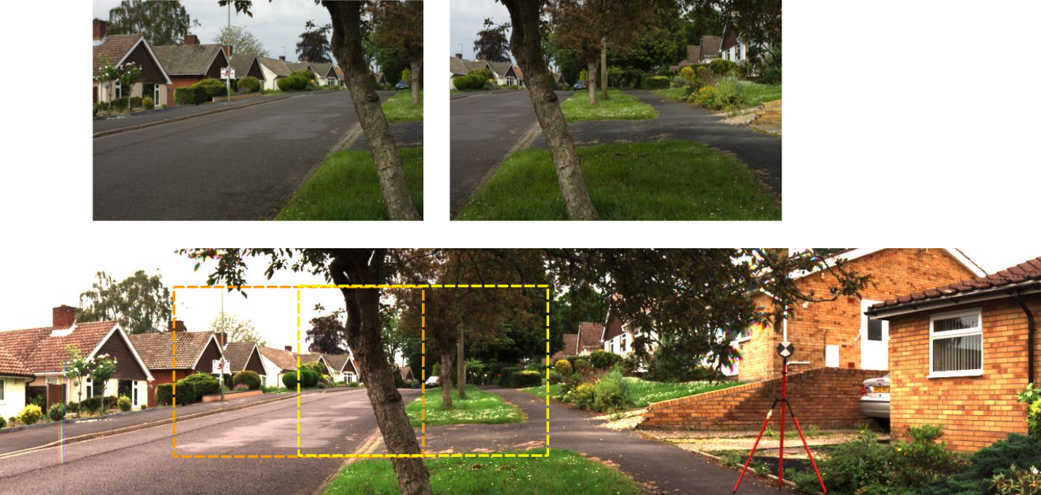
Figure 2: Section of panorama plus left-eye stereo images for views 1 and 2, scene 2.

Step 2

Reprojection of panorama.  Sections of the panorama (originally with equirectangular projection) were reprojected under cartesian projection to create 18 new ‘cyclopean images’, each corresponding to one of the 18 stereo images.  This step used the azimuth correspondence found in Step 1, alongside the field of view information for the stereo cameras, derived from calibration images. The cart2sph function was used to identify source pixels from the panorama for each pixel in the cyclopean image, and scatteredInterpolant was used to create the intensity values of new pixels at discrete locations in the cartesian image. The resultant cyclopean images were created with 1/8 resolution of the stereo images due to the comparatively low spatial resolution of the original panorama.

Step 3

Stereo-cyclopean image feature matching. To fine-tune the co-registration of the stereo and cyclopean images, image features were extracted and matched across the two images. To facilitate extraction of equivalent features in the two images, the images were first pre-processed: Both images were converted to greyscale, the stereo image was undistorted, using the known camera parameters (undistortImage) resized and then slightly blurred (imgaussfilt) to match the cyclopean image. Finally, to overcome the differences in luminance range and tone-mapping of the two images, the cyclopean image was adjusted using imhistmatch to match the distribution (maintaining ordinality) of the stereo image (Figure 3).

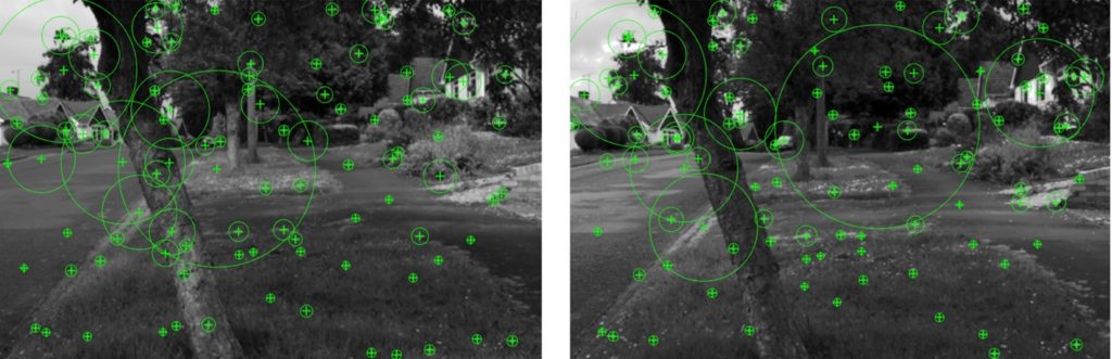
Figure 3. Cyclopean image reprojected from the panorama (left) and left image of stereo pair (right), each showing a random selection of 100 extracted (unmatched) features. Crosses give the feature location, and circles give the feature scale.  

Image features were identified iteratively (separately for each image) using detectSURFFeatures, reducing the threshold for feature detection until at least 400 were identified (typically many times that). The resultant features (Figure 3) were characterized (extractFeatures) and then matched across the two images (matchFeatures, Figure 4). Using the image locations of the matched features, the geometric transformation between the two cameras was determined (estimateFundamentalMatrix) and outlier matches (with non-trivial vertical disparities) were rejected. If less than 250 valid matched points remained, the process of matching and identifying features was repeated, with more lenient thresholds for identification and initial matching. After 10 such unsuccessful iterations, the scene & view was discarded. This failure occurred for scenes with predominantly homogenous textures, e.g. water and sky or grassy field and sky.

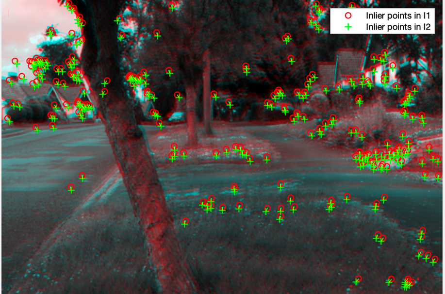
Figure 4. Matched features for the two images, shown as a red-blue ‘analgyph’.

Step 4

Find the world coordinates (x, y, z) of the matched features. Using the mapping between cyclopean and panorama images, the elevation and azimuth of each matched feature was found. With the panorama and LiDAR point cloud already co-registered, the LiDAR point closest to the centre of each image feature was identified (LiDAR has higher spatial resolution than panorama).

Step 5

Project LiDAR data to stereo image.  First, the precise position and orientation of the stereo camera, with respect to the LiDAR point cloud, was determined using estimateWorldCameraPose. The goodness of fit of the estimated camera pose was evaluated by the SSE of reprojected LiDAR points relative to the left eye’s image points (using cameraPoseToExtrinsics and worldToImage). A grid search of horizontal and vertical field of view parameters near to the nominal values identified the optimal camera pose estimate, i.e. that which minimised the SSE. Using the optimized camera pose estimate, the function worldToImage was used to project all LiDAR points within the appropriate region of point cloud to the image plane, to create the depth map.

The spatial resolution of the LiDAR data is not constant across the image plane, having its minimum at zero elevation. Accordingly, depth maps, with associated stereo image pairs are provided at two different spatial resolutions. The first, 600 x 900 (i.e. 0.15 scale of the original stereo images) ensures that all pixels within the depth map are filled (other than non-returns for sky, etc).  The second, 688 x 1032 provides more LiDAR depth points, but leaves a few undefined pixels in the periphery of the depth map.

Figure 5: Left eye’s stereo image, with re-projected LiDAR points. As can be seen, occasional false matches made it through the feature-matching process. Right image: depth map from LiDAR.

Step 6

LiDAR data and stereo images were captured sequentially. Thus, for some scenes, objects (e.g., cars, people) moved during the intervening minutes. For each of these scene views a depth mask was created to define these regions containing motion artefacts.

These regions were identified manually via inspection of a GIF created from the left stereo image and the LiDAR intensity data.